Spatial Altruism
Spatial Altruism is the minimal evolved-cooperation case study on this site. It asks a deceptively simple question: how can an altruistic inherited trait survive when selfish competitors enjoy the same local benefit without paying the altruist cost?
The page is easiest to read as a sequence: first the baseline case in which selfishness wins, then the local update rule that produces that result, then the harsher setting in which altruist clusters can survive better.
The Puzzle
If altruists help their neighborhood but selfish individuals get that help for free, selfishness should appear to have the direct advantage.
That is the starting puzzle of the model:
- altruists produce a shared local benefit,
- altruists alone pay the direct cost of producing it,
- selfish individuals can exploit that benefit without contributing.
So under ordinary dense conditions, selfish competitors should tend to win. Spatial Altruism asks whether that conclusion changes once reproduction is local and empty space becomes an active ecological competitor.
What Kind Of Model This Is
This is a patch-based evolutionary model of selection on inherited types, not a model of planning, reasoning, or within-lifetime learning.
It represents a spatial population in which:
- each grid cell is either empty or occupied by one individual,
- occupied cells come in two inherited types: altruist or selfish,
- reproduction is represented by a local replacement lottery for space,
- the composition of the population changes across generations.
One useful intuition is to imagine local plants, colonies, or lineages "seeding" for nearby space. Each occupied site contributes reproductive pressure toward itself and its neighbors, and the next occupant of each site is determined by a local genetic lottery. That setup is enough to generate the two comparisons that organize the page: the baseline outcome in Display 1 and the harsher empty-space regime in Display 2.
Display 1: The Baseline Result
Each patch has one of three visible states in the figures on this page and in the sampled browser replay:
- altruist: dark burgundy-red
- selfish: blue
- empty: light beige
Display 1 is the baseline run. It uses the same initial population mix as Display 2 and the replay below, but it does not give empty space any extra competitive help in the local lottery. The point of starting here is simple: in this baseline version, selfishness wins.
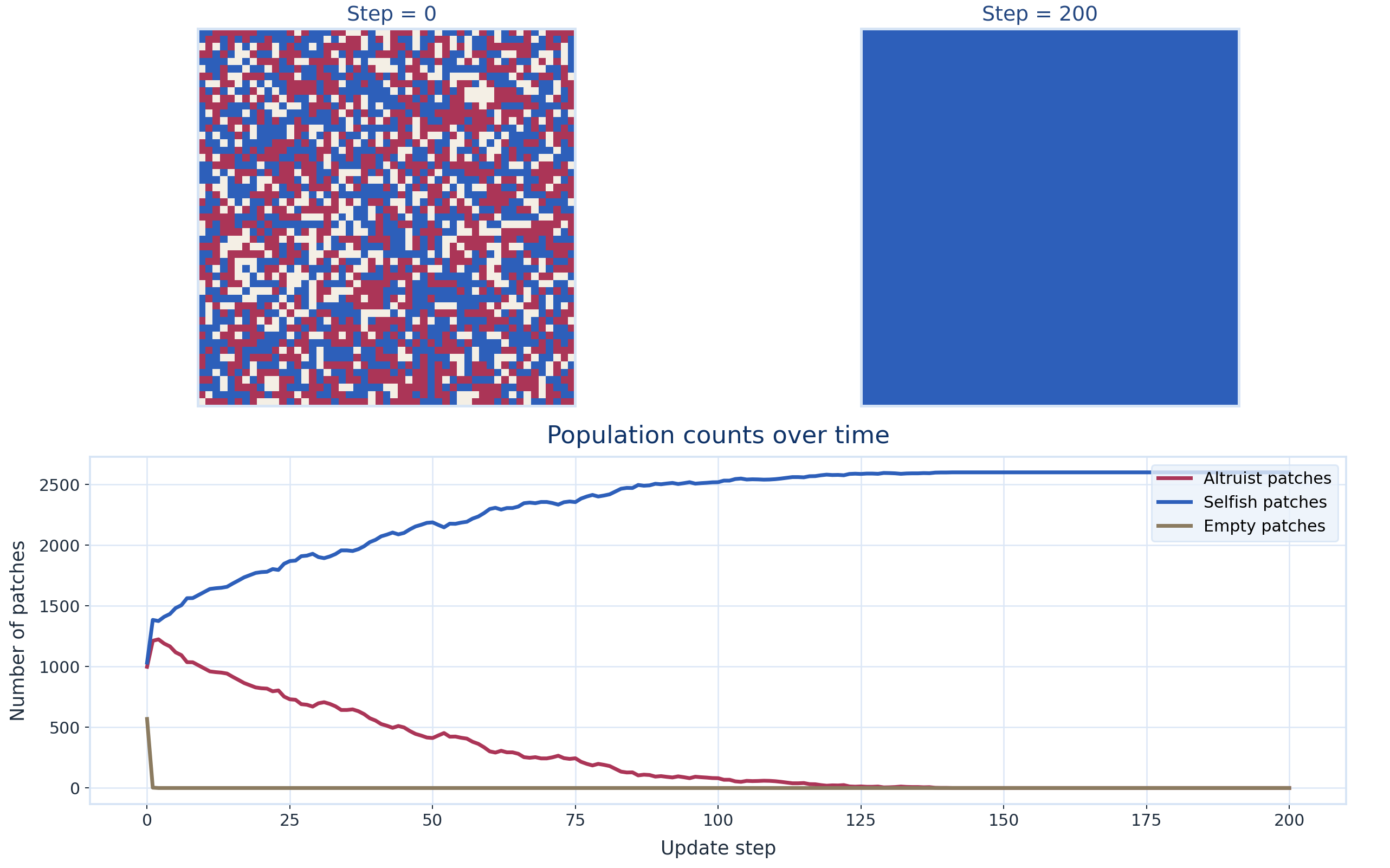
Two things are worth noticing immediately in Display 1:
- empty space disappears almost immediately,
- selfish patches steadily drive altruists to extinction.
That is the baseline story. If the main contest is just altruists versus selfish free-riders, selfishness takes over. In this baseline run, altruists start at 999 patches but fall to 81 by step 100 and to 0 by step 150, while selfish patches rise to 2601, the entire 51 × 51 world. The next step is to see how one update works, because that makes clear why the baseline behaves this way and why Display 2 behaves differently.
How One Update Works
Before introducing the exact notation later on, it helps to understand what one generation does.
- A focal site looks at a plus-shaped neighborhood of five sites: itself, up, down, left, and right.
- The number of nearby altruists determines how much local social benefit is available at that focal site.
- Each site in that neighborhood receives a fitness value: altruists pay a cost, selfish individuals do not, and empty sites may or may not receive their own competitive weight depending on the version of the model.
- Those fitness values are added by type to form a local lottery for who occupies the focal site next.
- In the Display 2 version, the void also receives an extra bonus term that makes emptiness more likely even when nearby occupied sites are strong.
- The next occupant of the focal site is sampled from those lottery weights.
The model is spatial because each focal site repeats that process using only its own plus-shaped neighborhood:
- the focal patch itself,
- the patch above,
- the patch below,
- the patch to the left,
- the patch to the right.
So each local calculation uses exactly 5 patches.
Display 1 and Display 2 use this same local update structure. The difference is that Display 1 leaves empty-space pressure turned off, while Display 2 turns it on strongly.
Why Display 2 Changes The Outcome
Display 2 changes one part of the selection environment: empty space becomes an active competitor in the local lottery.
Two terms do that work:
harshnessgives empty patches their own baseline competitive weightdiseaseadds extra lottery mass favoring emptiness on top of that baseline
That changes the question. In Display 1, the main issue is whether altruists or selfish free-riders win in a dense mixed world. In Display 2, the question becomes:
Which inherited type survives and regrows better when local neighborhoods are repeatedly thinned out by the void?
In the Display 2 setting, the answer is: altruist clusters survive that ecological filter better than selfish free-riders.
The logic is:
- selfish patches benefit from altruists only when altruists are nearby
- selfish patches do not help maintain those beneficial neighborhoods
- altruist clusters, by contrast, support one another's local fitness
- when the void expands, selfish patches lose the support structure they were exploiting
- clustered altruists are better able to hold or recolonize the remaining occupied pockets
This is why harshness and disease do not reward altruism directly. They reward whatever survives best against the void, and under these settings that favors clustered altruists.
The contrast is strong in the canonical code-backed counterfactuals for this same Display 2 parameterization:
- with
disease = 0.0, altruists are extinct by step200 - with
harshness = 0.0, altruists are also extinct by step200 - with both present in the Display 2 run, altruists survive and eventually dominate the remaining occupied sites
Display 2 shows that altered selection environment.
harshness = 0.96 and disease = 0.213), showing altruist survival under strong void pressure.Reading Display 2
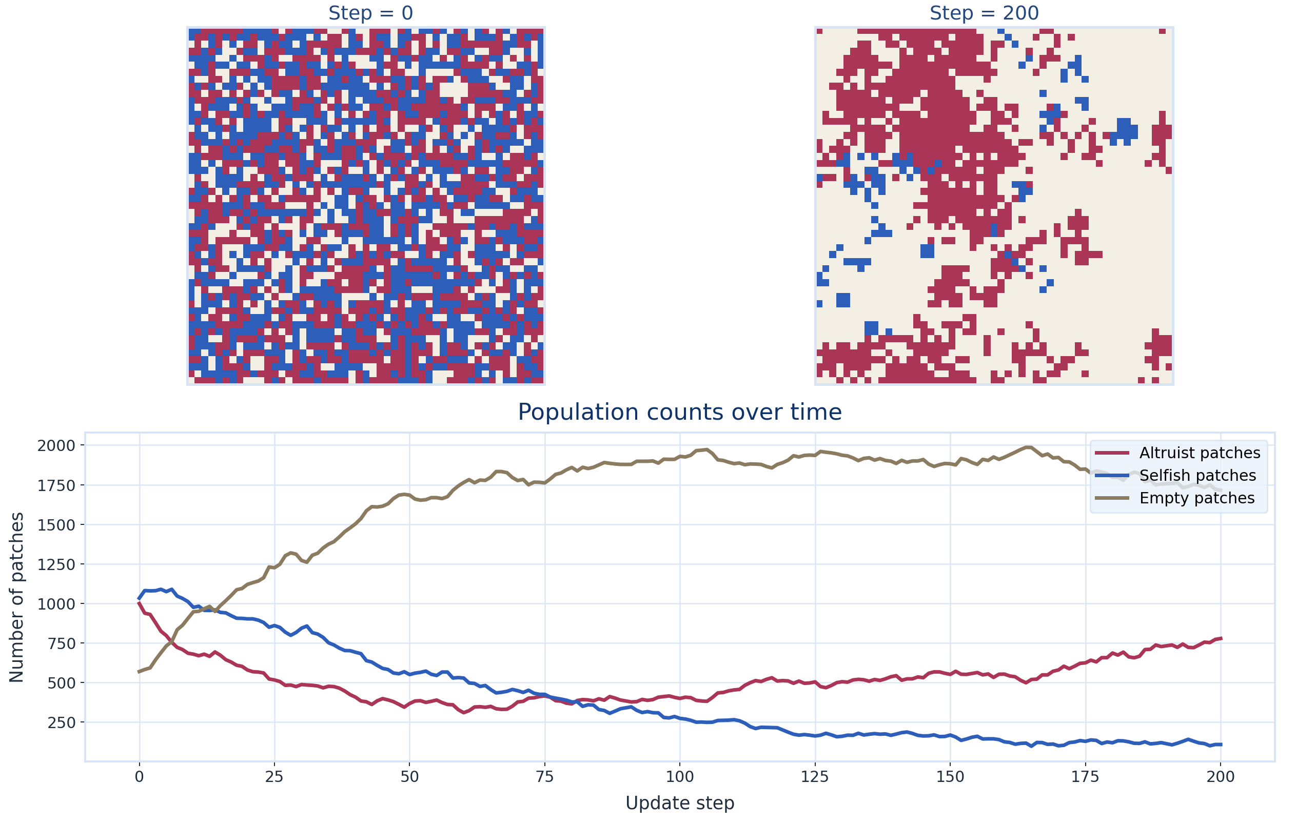
Display 2 is a specific seeded run, not a schematic sketch. It uses the same initial population mix as Display 1, but under much stronger empty-space pressure. The main settings are:
- initial
altruistic_probability = 0.39 - initial
selfish_probability = 0.39 benefit_from_altruism = 0.468cost_of_altruism = 0.156harshness = 0.96disease = 0.213seed = 1
The trajectory in the chart is easiest to read in three phases.
Phase 1: selfish patches lead in dense mixed regions
At the beginning, selfish patches exploit altruist-produced benefit without paying the altruist cost. In this run, altruists start at 999 patches and selfish patches at 1033, but by step 25 altruists have fallen to 516 while selfish patches remain higher at 860.
Phase 2: the void expands and occupancy collapses
Then the empty state begins winning many local lotteries. harshness = 0.96 makes empty sites almost as competitive as occupied ones even before the extra void term is added, and disease = 0.213 pushes the lottery further toward emptiness. That is why the beige region spreads so rapidly and why the empty-patch curve rises from 569 initially to 1684 by step 50, then to 1929 by step 100.
Phase 3: altruists survive better in the sparse regime
Once empty space dominates, selfish patches lose the altruist neighbors they were exploiting. Altruist clusters, by contrast, still support one another locally. So even though altruists lost ground early, they become the majority among the remaining occupied patches later on. In this run, altruists are only about 37.5% of occupied patches at step 25, but about 59.4% by step 100, 76.6% by step 150, and 87.8% by step 200.
So Display 2 is not showing altruism becoming intrinsically stronger than selfishness. It is showing the selection environment changing. In a dense mixed world selfishness wins locally; in a harsh, void-dominated world clustered altruists survive the ecological filter better.
Interactive Replay
The browser replay below is based on sampled frames from the same steady_state configuration shown in Display 2.
The canonical implementation and supporting analysis live in the EvolvedCooperation repository:
Evolved Cooperation
Spatial Altruism
Sampled browser replay of the Python model. The page renders the replay directly from a fixed exported run.
Replay
World State
Formal Ingredients
The story above is enough to follow the main argument of the page. The definitions below give the exact implementation and notation used by the underlying model.
Local Benefit Rule
The altruism benefit at one patch is:
altruism_benefit = benefit_from_altruism × (benefit_out_self + sum_of_neighbor_benefit_out) / 5
Variable meanings:
altruism_benefit: total social benefit currently available at the focal patchbenefit_from_altruism: strength of the positive externality produced by altruistsbenefit_out_self:1if the focal patch is altruist, otherwise0sum_of_neighbor_benefit_out: number of altruist contributors in the four-neighbor set5: the focal patch plus its four neighbors
This means altruists create a benefit that is local and shared.
Fitness Rule
Fitness depends on patch type:
- altruist patch:
fitness = (1 - cost_of_altruism) + altruism_benefit - selfish patch:
fitness = 1 + altruism_benefit - empty patch:
fitness = harshness
Variable meanings:
fitness: the reproductive weight a patch contributes to nearby lotteriescost_of_altruism: private cost paid only by altruist patchesharshness: baseline weight assigned to empty patches
This is the core social dilemma:
- altruists help the neighborhood,
- selfish patches enjoy that help too,
- but only altruists pay the direct cost.
Neighborhood Lottery
After each patch computes its fitness, the focal patch collects three local totals:
alt_fitness: summed fitness contributed by altruist patches in the focal plus-neighborhoodself_fitness: summed fitness contributed by selfish patches in the focal plus-neighborhoodharsh_fitness: summed fitness contributed by empty patches in the focal plus-neighborhood
The local competition neighborhood is always the same five-site plus shape, but the empty-site term depends on the model variant.
For steady_state:
alt_weight = alt_fitness / fitness_sumself_weight = self_fitness / fitness_sumharsh_weight = (harsh_fitness + disease) / fitness_sumfitness_sum = alt_fitness + self_fitness + harsh_fitness + disease
For uniform_culling and compact_swath:
alt_weight = alt_fitness / fitness_sumself_weight = self_fitness / fitness_sumharsh_weight = harsh_fitness / fitness_sumfitness_sum = alt_fitness + self_fitness + harsh_fitness
Variable meanings:
alt_weight: probability mass for the next patch becoming altruistself_weight: probability mass for the next patch becoming selfishharsh_weight: probability mass for the next patch becoming emptydisease: extra void lottery massxiused only insteady_state; the culling variants setdisease = 0.0
The next generation at each patch is then sampled from those weights:
- altruist if the draw lands in
alt_weight - selfish if the draw lands in
self_weight - empty otherwise
Both still figures on this page and the replay use that same plain steady_state rule. The difference is parameterization:
- Display 1 shows the baseline case with no extra competitive help for empty space
- Display 2 and the replay use the same initial population mix under strong
harshnessanddisease
The culling figures later on the page describe an extension of the model, not the mechanism shown in these steady-state displays.
Why This Belongs Under Evolved Cooperation
This model belongs under evolved cooperation because it studies cooperation through inherited variation and selection across generations.
Within the site's evolved-cooperation set, Spatial Altruism is the minimal local public-good benchmark.
| Case study | Selection logic |
|---|---|
| Spatial Altruism | A minimal patch-based model in which altruist and selfish traits compete through local benefit, private cost, and a neighborhood lottery. |
| Cooperative Hunting | A spatial ecological model in which predator cooperation evolves through hunting success, energetic cost, and inherited trait variation. |
| Spatial Prisoner's Dilemma | A local-game ecology in which inherited same-vs-other Prisoner's Dilemma response rules spread through energy accumulation, local movement, and local reproduction. |
| Retained Benefit | An abstract lattice model in which a continuous cooperation trait spreads only when enough of the value created by cooperation is routed back toward cooperators or copies of the cooperative rule. |
Culling Variants
The repository now implements the full three-variant Mitteldorf-Wilson set:
steady_state: void competition with continuous empty-patch lottery massuniform_culling: scheduled random evacuation of a fixed share of sitescompact_swath: scheduled clearing of one contiguous square region
The replay above remains a sampled steady_state run matching Display 2, but the underlying Python module also includes both disturbance variants.
Culling Experiment
A first culling-only sweep compared uniform_culling and compact_swath under the following settings:
benefit_from_altruismfrom0.00to1.00in steps of0.05cost_of_altruismfrom0.00to0.35in steps of0.05- fixed
harshness = 0.96 - disturbance interval
50 - disturbance fractions
0.25and0.50 - initial
altruistic_probability = 0.39 - initial
selfish_probability = 0.39 disease = 0.0because both runs use culling variants rather than the steady-state void-lottery term5replicates per parameter set- outcomes scored at step
1000
Headline outcome:
- both culling variants produced coexistence regions
uniform_cullingwas more robust overall thancompact_swath- the strongest gap appeared at disturbance fraction
0.50
Measured summary from that sweep:
- mean coexistence probability was about
0.089foruniform_cullingand0.057forcompact_swath - mean occupied fraction was about
0.509foruniform_cullingand0.400forcompact_swath - at disturbance fraction
0.50,uniform_cullingstill reached coexistence probability1.0, whilecompact_swathpeaked at0.8
Static Culling Heatmaps
The next figures fix harshness = 0.96, disturbance interval 50, and disturbance fraction 0.50. They compare the two disturbance variants over the benefit_from_altruism and cost_of_altruism plane.
Coexistence Probability
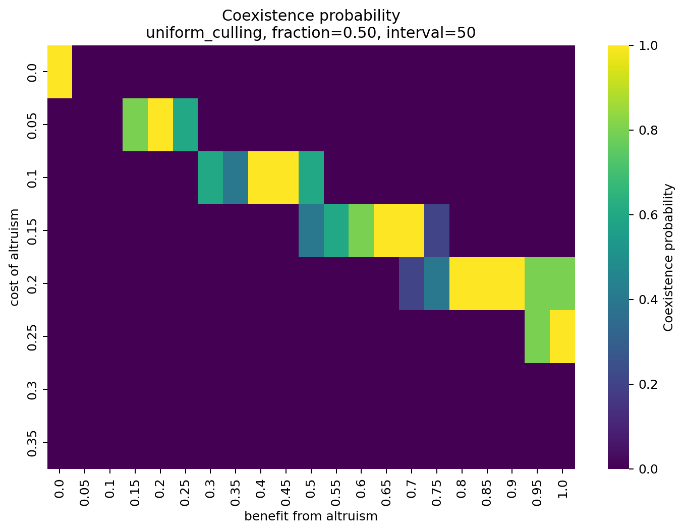
uniform_culling still shows parameter cells with coexistence probability 1.0 at disturbance fraction 0.50.
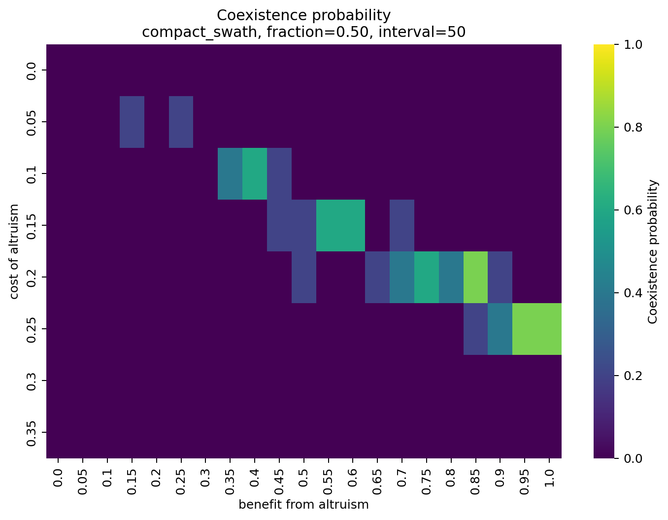
compact_swath retains coexistence in a narrower region and does not reach 1.0 at the same disturbance level in this sweep.
Occupied Fraction
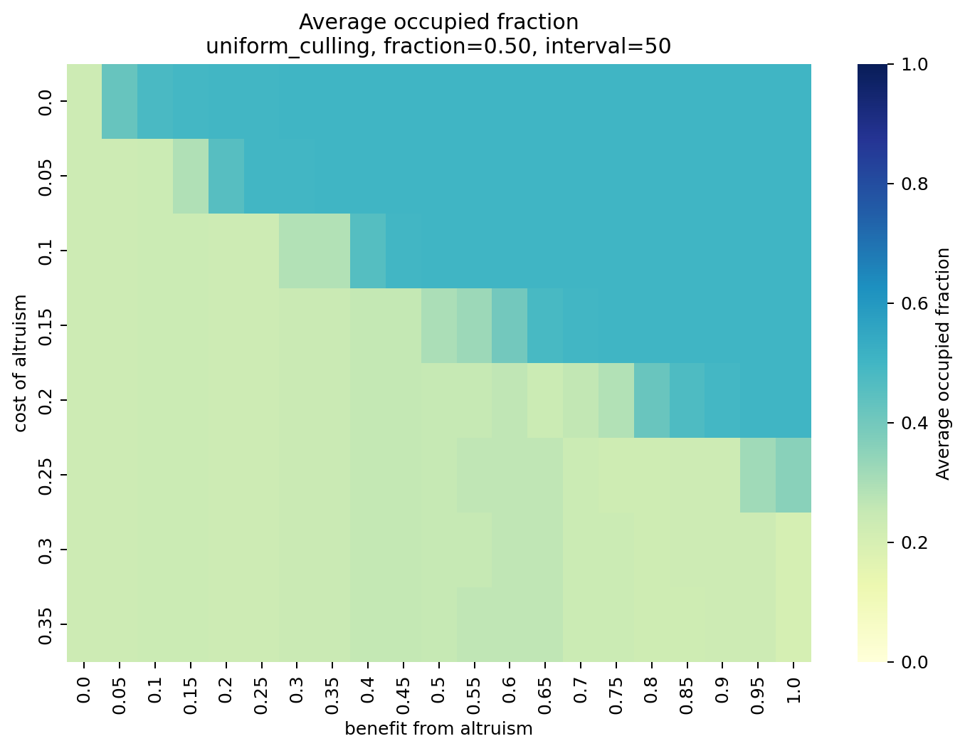
Under the same disturbance settings, uniform_culling preserves substantially more occupied space on average.
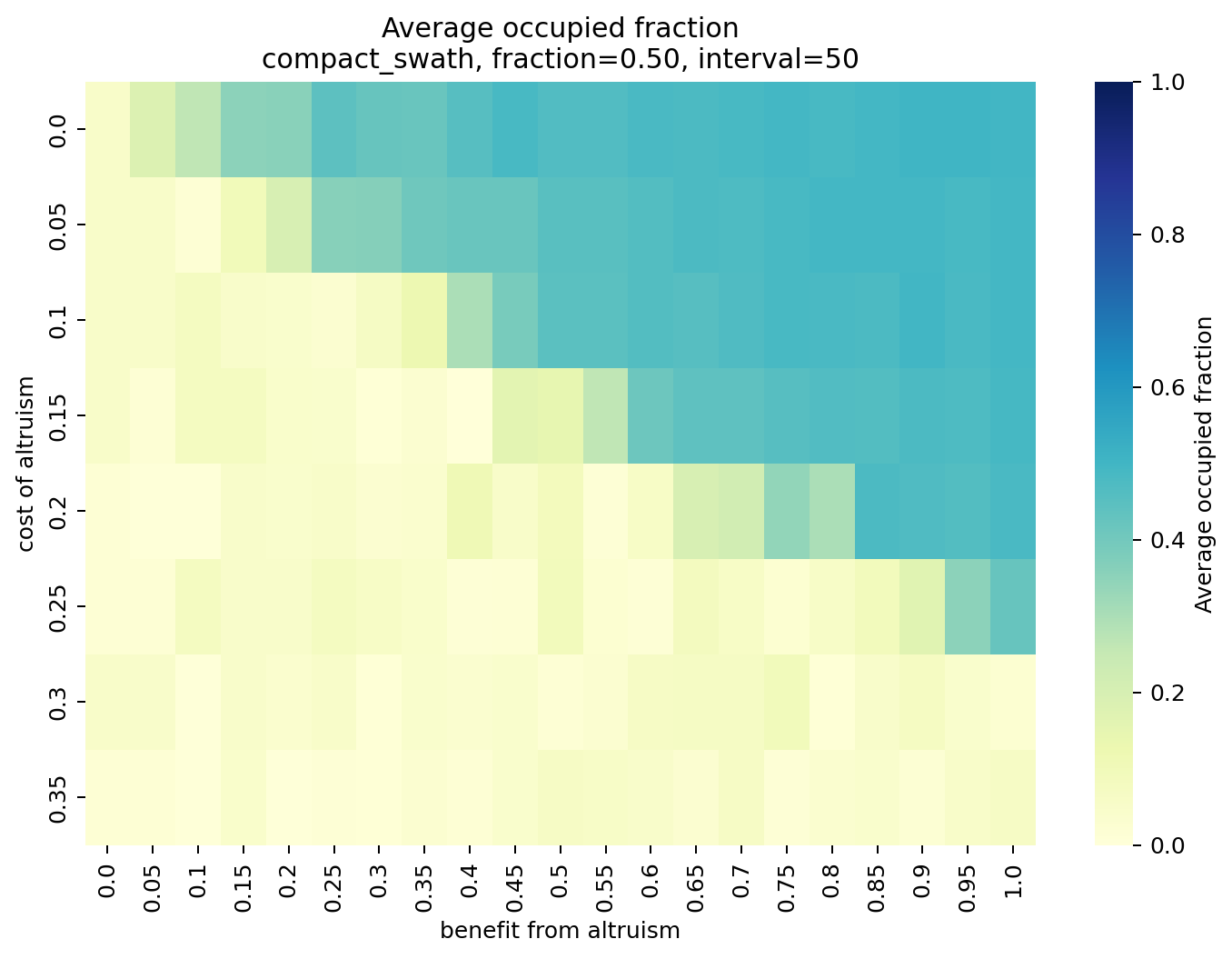
compact_swath produces a sharper occupancy collapse, consistent with a stronger recolonization bottleneck after contiguous clearing.
Conclusions
This case study gives a conditional answer to the question of how cooperation can emerge.
- cooperation does not emerge automatically just because helping produces a shared benefit; when cooperators and free-riders are mixed together in ordinary dense conditions, the free-riders win because they get the benefit without paying the cost
- cooperation becomes more likely when the environment changes who can survive and recover; in the harsher setting on this page, empty space expands and local clusters matter more, which helps groups of cooperators persist better than isolated free-riders
- the main lesson is that cooperation here is not favored because altruism is always stronger in itself; it is favored when ecological structure makes it harder for selfish individuals to keep exploiting cooperators
- more broadly, this means the emergence of cooperation depends on context: population structure, local interaction, and environmental pressure can change whether selfishness or cooperation is selected
- the culling results point in the same direction; disturbance can sometimes preserve coexistence, and scattered clearing was more supportive of coexistence than one large contiguous cleared region in this first sweep
- this is therefore not a claim that cooperation always evolves; it is a claim that cooperation can emerge when the environment and the spatial structure protect cooperative clusters long enough for selection to favor them
References
- Mitteldorf, J., & Wilson, D. S. (2000). Population viscosity and the evolution of altruism. Journal of Theoretical Biology, 204(4), 481-496. https://doi.org/10.1006/jtbi.2000.2007
- Wilensky, U. (1998). NetLogo Altruism model. http://ccl.northwestern.edu/netlogo/models/Altruism. Center for Connected Learning and Computer-Based Modeling, Northwestern University, Evanston, IL. A NetLogo implementation of the Mitteldorf & Wilson paper: Altruism model (
Altruism.nlogox), Curricular Models / BEAGLE Evolution / EACH. https://www.netlogoweb.org/launch#https://www.netlogoweb.org/assets/modelslib/Curricular%20Models/BEAGLE%20Evolution/EACH/Altruism.nlogox EvolvedCooperation. spatial_altruism module directory. GitHub. https://github.com/doesburg11/EvolvedCooperation/tree/main/spatial_altruismEvolvedCooperation. spatial_altruism/altruism_model.py. GitHub. https://github.com/doesburg11/EvolvedCooperation/blob/main/spatial_altruism/altruism_model.pyEvolvedCooperation. spatial_altruism/README.md. GitHub. https://github.com/doesburg11/EvolvedCooperation/blob/main/spatial_altruism/README.md